Challenges of Score Matching

Introduction

Modern day models are incredibly rich and expressive, powering contemporary advances in machine learning and statistical inference. The idea of modelling is that we are given some data X_1, \ldots, X_n \in \mathcal X and want to get a handle on the underlying distribution that generates the data. To do this, one approach is parametric inference: we take a family of distributions \mathcal Q= \left\{ q_{\theta} \colon \theta \in \Theta \right\} indexed by a parameter \theta \in \Theta. We assume for simplicity that X_1, \ldots, X_n are drawn i.i.d. from q_{\theta^\star} for some true parameter \theta^\star where \theta^\star \in \Theta. Based on our data, we seek to produce an estimate \hat \theta of the true parameter \theta^\star.

Maximum likelihood estimation

One such estimate is the maximum likelihood estimate (MLE), which is the element of \Theta that maximizes the likelihood (or equivalently log-likelihood) of the data: \begin{aligned} \hat \theta_{\text{MLE}} \overset{\mathrm{def}}{=}\mathop{\mathrm{arg max}}_{\theta \in \Theta} \prod_{i=1}^{n} q_\theta(X_i) = \mathop{\mathrm{arg max}}_{\theta \in \Theta} \frac{1}{n} \sum_{i=1}^{n} \underbrace{\log q_\theta(X_i)}_{\overset{\mathrm{def}}{=}\ell(\theta; X_i)}. \end{aligned} As n \to \infty, by the Law of Large Numbers, we have that \begin{aligned} \frac{1}{n} \sum_{i=1}^{n} \ell(\theta; X_i) \overset{\mathbb P}{\to} \mathbb E[\ell(\theta; X_1)] = \mathbb E[\log q_\theta(X_1)]. \end{aligned} On the other hand, we have that \begin{aligned} \mathbb E[\log q_{\theta^\star}(X_1)] - \mathbb E[\log q_{\theta}(X_1)] = \mathbb E\left[ \log \frac{q_{\theta^\star}}{q_{\theta}}(X_1) \right] = \mathsf{KL}\left(q_{\theta^\star} \,\Vert\, q_{\theta}\right), \end{aligned} where \mathsf{KL}\left(p \,\Vert\, q\right) denotes the KL divergence between distributions p and q. The KL divergence between two distinct distributions is positive, meaning that for any \theta, \theta^\star for which q_\theta \neq q_{\theta^\star}, we have \mathsf{KL}\left(q_{\theta^\star} \,\Vert\, q_\theta\right) > 0. So as n \to \infty, the MLE \hat \theta_{\text{MLE}} will converge in probability to the true parameter \theta^\star: in other words, the MLE is a consistent estimator. Furthermore, the MLE is asymptotically efficient: that is, no other estimator attains a strictly lower variance than the MLE as n \to \infty.

However, the richness of models comes at a cost. Often, the parameterized distribution q_\theta can only be specified up to a constant of proportionality. For instance, we might specify that q_\theta(x) \propto \exp(-V_\theta(x)) for some log-potential function V_\theta \colon \mathcal X\to \mathbb R. Since q_{\theta} is a probability distribution, it must sum to 1, meaning that we have \begin{aligned} q_{\theta} = \frac{\exp(-V_\theta(x))}{Z(\theta)}, \qquad \text{where} \; Z(\theta) \overset{\mathrm{def}}{=}\int_{\mathcal X} \exp(-V_{\theta}(x'))\,\mathrm{d}{x'}. \end{aligned} The issue is that for each value of \theta, there is a different normalization constant Z(\theta), and computing even a single normalization constant is generally intractable when the data space \mathcal X is large. Computing the MLE falls victim to this issue: if we cannot compute Z(\theta), then there is no hope of computing \hat \theta_{\text{MLE}} because the objective function depends on the value of Z(\theta).

Score matching

The score matching estimator (SME), introduced by Hyvärinen (2005), promises to solve this issue. The SME is defined by \begin{aligned} \hat \theta _{\text{SME}} \overset{\mathrm{def}}{=}\mathop{\mathrm{arg min}}_{\theta \in \Theta} \frac{1}{n} \sum_{i=1}^{n} \biggl[ \underbrace{ \mathop{\mathrm{Tr}}(\nabla^2 \log q_\theta (X_i)) + \frac{1}{2}\left\lVert \nabla \log q_\theta(X_i) \right\rVert^2 }_{\overset{\mathrm{def}}{=}\varphi (\theta; X_i)} \biggr]. \end{aligned} The quantity \nabla \log q_\theta is known as the score function of q_\theta. Since the gradient is taken with respect to x rather than \theta, the normalization constant vanishes altogether from the objective function: hence, the score matching estimator indeed evades the need to normalize, giving it one computational advantage over the MLE.

Now the question is: is this estimator any good? How do its statistical properties compare to the MLE?

As a first consideration, the SME is indeed a consistent estimator, just like the MLE. Indeed, we have that by the Law of Large Numbers, \begin{aligned} \frac{1}{n} \sum_{i=1}^{n} \rho(\theta; X_i) &= \frac{1}{n} \sum_{i=1}^{n} \left[ \mathop{\mathrm{Tr}}(\nabla^2 \log q_\theta (X_i)) + \frac{1}{2}\left\lVert \nabla \log q_\theta(X_i) \right\rVert^2 \right] \\ &\overset{\mathbb P}{\to} \mathbb E \left[ \mathop{\mathrm{Tr}}(\nabla^2 \log q_\theta (X_1)) + \frac{1}{2}\left\lVert \nabla \log q_\theta(X_1) \right\rVert^2 \right] \\ &= \frac{1}{2}\Bigl(\underbrace{ \mathbb E\left\lVert \nabla \log \frac{q_{\theta^\star}}{q_\theta}(X_1) \right\rVert^2 }_{= \mathsf{FI}\left(q_{\theta^\star} \,\Vert\, q_\theta\right)} - \mathbb E\left\lVert \nabla \log q_{\theta^\star}(X_1) \right\rVert^2 \Bigr) , \end{aligned} where the last equality follows by integration by parts. The first term on the last line is the relative Fisher information (FI) between q_{\theta^\star} and q_{\theta}, and is nonnegative with equality iff q_{\theta^\star} = q_\theta. Hence, asymptotically \theta^\star attains minimality of the objective, meaning that \hat \theta_{\text{SME}} is indeed consistent.

The story thus far looks good. Not only does the SME relieve the computational burden of evaluating the normalization constant, but it also provides a consistent estimator. Might it be the case that we can always just use the SME instead of the MLE?

Unfortunately, we must dash our hopes. The core idea of score matching is that if the score functions \nabla \log q_{\theta^\star} and \nabla \log q_{\theta} match exactly, then the distributions q_{\theta^\star} and q_{\theta} must match as well. However, there is a key issue. The score function, being a gradient, is fundamentally a measure of local information about the change in the log-likelihood function. Meanwhile, it is possible for two very different distributions to have extremely similar log-likelihood functions (up to a constant shift) outside of a set of very small measure. Until enough samples land in that distinguishing set, score matching cannot discern the difference between these two distributions.

This is the key intuition behind the statistical inefficiency of score matching: when \left\{ q_{\theta} \right\} is a family of distributions exhibiting the aforementioned behavior — having similar score functions outside a set of negligible measure — the SME can have extremely high variance compared with the MLE. As it turns out, this behavior is deeply related to the maximal log-Sobolev constant among distributions in \left\{ q_\theta \right\}; see the work of Koehler, Heckett, and Risteski (2022) for a discussion.

In the sequel, we will make our intuitive argument concrete by demonstrating that score matching is indeed statistically inefficient on a simple example of mixtures of well-separated Gaussians — a prototypical example of a distribution with large log-Sobolev constant.

Inefficiency for Mixtures of Gaussians

Let m > 0 be a mean parameter and p \in [0, 1] be a weight parameter. Define the Gaussian measures \mu_+ = \mathcal N(m, 1) and \mu_- = \mathcal N(-m, 1), and let \mu_p be the Gaussian mixture distribution defined by \mu_p = p \mu_+ + (1 - p) \mu_-. Then the score matching estimator \hat p_{\text{SME}} for p based on samples X_1, \ldots, X_n \overset{\mathrm{i.i.d.}}\sim\mu_p is given by: \begin{aligned} \hat p_{\text{SME}} = \mathop{\mathrm{arg min}}_{p \in [0, 1]} \frac{1}{n} \sum_{i=1}^{n} \bigl[ \nabla^2 \log \mu_p (X_i) + \frac{1}{2}(\nabla \log \mu_p (X_i))^2 \bigr]. \end{aligned} On the other hand, the MLE is given by \begin{aligned} \hat p_{\text{MLE}} = \mathop{\mathrm{arg min}}_{p \in [0, 1]} \frac{1}{n} \sum_{i=1}^{n} \log \mu_p (X_i) . \end{aligned}

Inefficiency of score matching

The following theorem shows that the SME is statistically inefficient compared to the MLE for learning the parameter p:

Theorem 1 (Inefficiency of score matching) Suppose that p^\star = \frac{1}{2} and that X \sim \mu_{p^\star}. Then as n \to \infty, we have that \begin{aligned} {\sqrt{n}} (\hat p_{\text{SME}} - p^\star) \overset{\text{D}}{\to} \mathcal N(0, \sigma^2_{\text{SME}}(m)), \end{aligned} where \sigma^2_{\text{SME}}(m) \in \Omega(m^2 e^{-\frac{1}{2}m^2}). On the other hand, \begin{aligned} {\sqrt{n}} (\hat p_{\text{MLE}} - p^\star) \overset{\text{D}}{\to} \mathcal N\left( 0, \sigma^2_{\text{MLE}}(m) \right), \end{aligned} where \sigma^2_{\text{MLE}}(m) \in O(1).

Hence, this example of learning the weight parameter of a mixture of one-dimensional standard Gaussians demonstrates an extreme gap in the statistical efficiency of the SME versus the MLE: the standardized asymptotic variance of the SME grows as e^{\frac{1}{2}m^2} whereas that of the MLE does not grow at all (in fact, shrinks)! The idea is that the MLE learns the weight parameter very easily by simply looking at the proportion of samples landing in the positive real axis versus the negative real axis, and high separation only makes this learning task easier. On the other hand, the SME suffers from the issue we posited earlier: the score functions \nabla \log \mu_p basically do not differ at all except on a small interval around 0, and the measure of this set is extremely small, on the order of e^{-\frac{1}{2}m^2}.

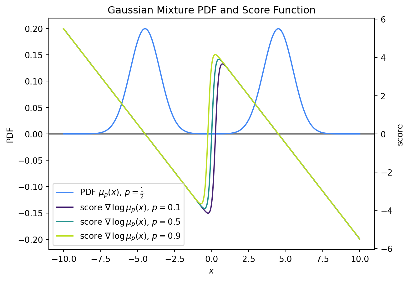
In Section 3.1, we compute the score function \nabla \log \mu_p as well as its partial derivatives with respect to p. Using these formulas, we can obtain our desired bounds. On the other hand, before diving into the proof, we first provide an illustration in Figure 1 that confirms our above intuition.

Visualizing score function for varying p

We plot the score functions \nabla \log \mu_p (x) with m = 4.5 for p \in \{0.1, 0.5, 0.9\}, superimposing the mixture PDF to visually demonstrate that the score functions only vary significantly on a set of negligible measure.

Code

import numpy as np
import matplotlib.pyplot as plt
import warnings
warnings.filterwarnings("ignore")

def gaussian_pdf(x, mean, sigma):
    return (
      1 / (sigma * np.sqrt(2 * np.pi)) *
      np.exp(-(x - mean) ** 2 / (2 * sigma ** 2))
    )

def mixture_pdf(x, mean, sigma, p):
    # Mixture with weights p
    mu_plus = gaussian_pdf(x, mean, sigma)
    mu_minus = gaussian_pdf(x, -mean, sigma)
    return (p * mu_plus + (1-p) * mu_minus)

def score_function(x, mean, sigma, p):
    mu_plus = gaussian_pdf(x, mean, sigma)
    mu_minus = gaussian_pdf(x, -mean, sigma)
    pos = p * mu_plus * (- x + mean) / (sigma ** 2)
    neg = (1-p) * mu_minus * (- x - mean) / (sigma ** 2)
    return (pos + neg) / (mixture_pdf(x, mean, sigma, p))

x = np.linspace(-10, 10, 1000)

# set the mean and std
mean = 4.5
sigma = 1

# Set the weight parameter for the Gaussian mixture
p = 0.5  # Equal weights for the two Gaussians

# Compute the PDF and score function for each x value
pdf = mixture_pdf(x, mean, sigma, p)

# Plotting the Gaussian mixture PDF and score function
fig, ax1 = plt.subplots()
blue = '#4287f5'
ax1.axhline(0, color='gray')
ax1.plot(x, pdf, blue, label=r'PDF $\mu_{p}(x)$, $p = \frac{1}{2}$')
ax1.set_xlabel(r'$x$')
ax1.set_ylabel('PDF')
ax1.tick_params(axis='y')

# Set symmetric y limits on left
y_min, y_max = -np.max(pdf) * 1.1, np.max(pdf) * 1.1
ax1.set_ylim(y_min, y_max)

# Plot score functions for different values of p
ax2 = ax1.twinx()
for p in np.linspace(0.1, 0.9, 3):
  color = plt.cm.viridis(p)
  scores = score_function(x, mean, sigma, p)
  ax2.plot(x, scores, color=color, label=fr'score $\nabla \,\log \mu_{{p}}(x)$, $p={p}$', )
ax2.set_ylabel('score')
ax2.tick_params(axis='y')

# Display legend
lines = ax1.get_lines() + ax2.get_lines()
plt.legend(lines, [line.get_label() for line in lines], loc='lower left')

plt.title('Gaussian Mixture PDF and Score Function')
plt.show()

Figure 1: The score function varies negligibly with p outside a set of extremely small measure. Hence, learning p via score matching should be extremely sample inefficient.

Proof

Proof (Theorem 1). Define the risk function \begin{aligned} \varphi(p; x) &= \nabla^2 \log \mu_p (x) + \frac{1}{2}(\nabla \log \mu_p (x))^2, \end{aligned} so that \begin{aligned} \hat p_{\text{SME}} = \mathop{\mathrm{arg min}}_{p \in [0, 1]} \frac{1}{n} \sum_{i=1}^{n} \varphi(p, X_i) . \end{aligned} Furthermore, denote \begin{aligned} \varphi_n(p) \overset{\mathrm{def}}{=} \frac{1}{n} \sum_{i=1}^{n} \varphi(p, X_i). \end{aligned} Now, since the SME is consistent, \hat p_{\text{SME}} will be close to p^\star as n \to \infty. This motivates performing a Taylor expansion of the objective function to obtain that \begin{aligned} 0 &= \partial_p \varphi_n (\hat p_{\text{SME}}) \approx \partial_p \varphi_n (p^\star) + \partial_p^2 \varphi_n (p^\star) (\hat p_{\text{SME}} - p^\star). \end{aligned} Rearranging, we obtain that \begin{aligned} \sqrt{n}(\hat p_{\text{SME}} - p^\star) \approx \frac{\sqrt{n} \partial_p \varphi_n (p^\star)}{\partial_p^2 \varphi_n (p^\star)}. \end{aligned} Let X \sim \mu_{p^\star}. As n \to \infty, the Central Limit Theorem tells us that \begin{aligned} \sqrt{n} \partial_p \varphi_n (p^\star) \overset{\text{D}}{\to} \mathcal N(0, \mathop{\mathrm{Var}}\left[ \partial_p \varphi(p; X) \right]) = \mathcal N(0, \mathbb E\left[ (\partial_p \varphi(p^\star; X))^2 \right]), \end{aligned} where the last equality is due to the fact \partial_p \,\big\vert_{p = p^\star}\mathbb E[\varphi(p^\star; X)] = 0 due to asymptotic consistency. On the other hand, by the Law of Large Numbers, the denominator converges to \begin{aligned} \partial_p^2 \varphi_n(p^\star) = \mathbb E\left[ \partial_p^2 \varphi(p^\star; X) \right]. \end{aligned} Thus, we have that \begin{aligned} \sqrt{n}(\hat p - p^\star) \overset{\text{D}}{\to} \mathcal N\left( 0, \frac{\mathbb E\left[ \left( \partial_p \varphi(p; X) \right)^2 \right]}{\mathbb E\left[ \partial_p^2 \varphi(p; X) \right]^2} \right). \end{aligned} In fact, we can simplify the denominator of the variance expression. We have that \begin{aligned} \mathbb E\left[ \partial_p^2 \varphi(p; X) \right] &= \int \partial_p^2 \varphi(p; x) \,\mathrm{d}{\mu_p(x)}\\ &= -\int \partial_p \varphi(p; x) (\partial_p \mu_p(x))\,\mathrm{d}{x} \\ &= -\int \partial_p \varphi(p; x) \left( \frac{\partial_p \mu_p(x)}{\mu_p(x)} \right)\,\mathrm{d}{\mu_p(x)}\\ &= -\int (\partial_p \varphi(p; x)) (\partial_p \log \mu_p (x)) \,\mathrm{d}{\mu_p(x)}, \end{aligned} where the second equality is by integration by parts. Hence, \begin{aligned} \mathbb E\left[ \partial_p^2 \varphi(p; X) \right]^2 &= \mathbb E\left[ \partial_p \varphi(p; X) (\partial_p \log \mu_p (x)) \right]^2. \end{aligned}

Computing the partial derivative of the risk function with respect to p, we obtain that \begin{aligned} \partial_p \varphi(p; X) &= \partial_p \nabla^2 \log \mu_p (X) + (\nabla \log \mu_p(X)) (\partial_p \nabla \log \mu_p(X)). \end{aligned}

Now, we provide a lower bound on the numerator and an upper bound on the denominator as follows.

Lower bound on numerator.

Using the calculations in Section 3.1, we compute that \begin{aligned} \left\lvert \partial_p \varphi(p; X) \right\rvert &= \left\lvert \partial_p \nabla^2 \log \mu_p (X) + (\nabla \log \mu_p(X)) (\partial_p \nabla \log \mu_p(X)) \right\rvert \\ &= \left\lvert -\frac{16m^2}{(e^{mX} + e^{-mX})^2} \cdot \tanh(mX) + (-X + m \tanh(mX)) \cdot \frac{8m}{(e^{mX} + e^{-mX})^2} \right\rvert \\ &= \frac{8m}{(e^{mX} + e^{-mX})^2} \cdot \left\lvert X + m \cdot \tanh(mX) \right\rvert. \end{aligned} Consider when \left\lvert X \right\rvert \in [\frac{1}{2m}, \frac{1}{m}]. On this interval, we have that \begin{aligned} \frac{\left\lvert X + m \cdot \tanh(mX) \right\rvert}{(e^{mX} + e^{-mX})^2} &\geq \frac{m \left\lvert \tanh(mX) \right\rvert - \left\lvert X \right\rvert}{(e^{mX} + e^{-mX})^2} \\ &\geq \frac{m \tanh (1) - \frac{1}{m}}{(e + e^{-1})^2} \\ &\gtrsim m, \end{aligned} where the second inequality is a consequence of the triangle inequality. Thus, on this interval, we have that \begin{aligned} \left\lvert \partial_p \varphi(p; X) \right\rvert = \frac{8m\left\lvert X + m \cdot \tanh(mX) \right\rvert}{(e^{mX} + e^{-mX})^2} \gtrsim m^2. \end{aligned} Hence, we obtain that \begin{aligned} \mathbb E\left[ \left( \partial_p \varphi(p; X) \right)^2 \right] &= \mathbb E\left[ \left\lvert \partial_p \varphi(p; X) \right\rvert^2 \right] \\ &\geq \mathbb E\left[ \left\lvert \partial_p \varphi(p; X) \right\rvert^2 \mathbf 1_{\left\lvert X \right\rvert\in [\frac{1}{2m}, \frac{1}{m}]} \right] \\ &\gtrsim \mathbb E\left[ m^4 \mathbf 1_{\left\lvert X \right\rvert\leq [\frac{1}{2m}, \frac{1}{m}]} \right] \\ &\gtrsim m^4 e^{-\frac{1}{2}m^2}. \end{aligned}

Upper bound on denominator.

First, using the work above, we have that \begin{aligned} \left\lvert \partial_p \varphi(p; X) \right\rvert &= \frac{8m}{(e^{mX} + e^{-mX})^2} \cdot \left\lvert X + m \cdot \tanh(mX) \right\rvert \\ &\leq \frac{8m}{(e^{mX} + e^{-mX})^2} \cdot \left( \left\lvert X \right\rvert + m \right), \end{aligned} by the triangle inequality. On the other hand, using Section 3.1, we compute that \begin{aligned} \left\lvert \partial_p \log \mu_p (X) \right\rvert &= \left\lvert 2\tanh(mX) \right\rvert \leq 2. \end{aligned} Hence, we find that \begin{aligned} \mathbb E\left[ (\partial_p \varphi(p; X)) (\partial_p \log \mu_p (X)) \right] &\leq \mathbb E\left[ \left\lvert \partial_p \varphi(p; X) \right\rvert \left\lvert \partial_p \log \mu_p (X) \right\rvert \right] \\ &\leq 2 \mathbb E\left[ \left\lvert \partial_p \varphi(p; X) \right\rvert \right] \\ &\lesssim \mathbb E\left[ \frac{m}{(e^{mX} + e^{-mX})^2} \cdot \left( \left\lvert X \right\rvert + m \right) \right] \\ &\lesssim m \int_{0}^{\infty} \frac{x + m}{(e^{mx} + e^{-mx})^2} \cdot e^{-\frac{1}{2}(x - m)^2} \,\mathrm{d}{x} \\ &\leq m \int_{0}^{\infty} \left( x + m \right) e^{-\frac{1}{2}(x - m)^2-2mx} \,\mathrm{d}{x} \\ &\lesssim me^{-\frac{1}{2}m^2}, \end{aligned} where the last equality is a consequence of Mills’ inequality (a tail bound on the Gaussian CDF).

Combining the upper and lower bounds, we find that the asymptotic variance of the score matching estimator is \begin{aligned} \frac{\mathbb E\left[ \left( \partial_p \varphi(p; Y, Z) \right)^2 \right]}{\mathbb E\left[ \partial_p^2 \varphi(p; Y, Z) \right]^2} &\gtrsim \frac{m^4 e^{-\frac{1}{2}m^2}}{\left( me^{-\frac{1}{2}m^2} \right)^2} \gtrsim m^2 e^{\frac{1}{2}m^2}. \end{aligned} This shows that the asymptotic variance grows as \Omega\left( m^2 e^{\frac{1}{2}m^2} \right), proving our desired result. Note that this is unbounded as a function of m!

On the other hand, let \ell(p; X) \overset{\mathrm{def}}{=}\log \mu_p(X), and let \ell'(p; X) \overset{\mathrm{def}}{=}\partial_p \ell(p; X). It is well-known that \begin{aligned} \sqrt{n}(\hat p_{\text{MLE}} - p^\star) \overset{\text{D}}{\to} \mathcal N\left( 0, \frac{1}{\mathbb E[\ell'(p^\star; X)^2]} \right). \end{aligned} Meanwhile, we compute that \begin{aligned} \mathbb{E}[\ell'(p^\star; X)^2] &= \int \frac{(\mu_+(X) - \mu_-(X))^2}{\mu_p(X)} \\ &= 2\int \frac{(\mu_+(X) - \mu_-(X))^2}{\mu_+(X) + \mu_-(X)}\\ &= 2\left( \int \frac{(\mu_+(X) + \mu_-(X))^2 - 4 \mu_+(X)\mu_-(X)}{\mu_+(X) + \mu_-(X)} \right) \\ &\geq 4\left( 1-2\int \frac{\mu_+(X)\mu_-(X)}{\mu_+(X)+\mu_-(X)} \right) \\ &\geq 4\left( 1-\int_+ \frac{\mu_+(X)\mu_-(X)}{\mu_+(X)} - \int_- \frac{\mu_+(X)\mu_-(X)}{\mu_-(X)} \right) \\ &\geq 4\left( 1-2\mathbb{P}(X \geq m) \right) \\ &\geq 4\left( 1 - \frac{1}{\sqrt{1 + m^2}}\exp\left( -\frac{m^2}{2} \right) \right), \end{aligned} where we have used Mills’ inequality to lower bound the Gaussian CDF. Hence, we obtain that the rescaled asymptotic variance of the MLE is bounded by \begin{aligned} \sigma^2_{\text{MLE}}(m) &= \frac{1}{\mathbb E[\ell'(p^\star; X)^2]} \leq \frac{1}{ 4\left( 1 - \frac{e^{-\frac{1}{2}m^2}}{\sqrt{1+m^2}} \right) }, \end{aligned} as desired.

Having shown both claims in the theorem, we conclude our proof. ◻

Appendix

Computation of score function derivatives

General case

First, we note that \begin{aligned} \nabla \log \mu_p = \frac{\nabla \mu_p}{\mu_p} = \frac{p \nabla \mu_+ + (1 - p) \nabla \mu_-}{p \mu_+ + (1 - p) \mu_-}\,. \nonumber \end{aligned} From this, we can compute the partial derivatives of the log-likelihood and score function with respect to p: \begin{aligned} \partial_p \log \mu_p &= 2\frac{\mu_+ - \mu_-}{\mu_+ + \mu_-} \nonumber \\ \partial_p \nabla \log \mu_p &= \frac{\mu_p(\nabla \mu_+ - \nabla \mu_-) - (\nabla \mu_p)(\mu_+ - \mu_-)}{\mu_p^2} \nonumber % \\ % \partial_p^2 \nabla \log \mu_p % &= % -2\frac{(\mu_+ - \mu_-)(\mu_p(\nabla \mu_+ - \nabla \mu_-) - (\nabla \mu_p)(\mu_+ - \mu_-))}{\mu_p^3}\,. % \nonumber \end{aligned}

Special case p = \frac{1}{2}

Specializing these formulas to the case p = \frac{1}{2}, we obtain that \begin{aligned} \partial_p \log \mu_p\,\big\vert_{p = \frac{1}{2}} &= 2\frac{\mu_+ - \mu_-}{\mu_+ + \mu_-} \nonumber \\ \nabla \log \mu_p \,\big\vert_{p = \frac{1}{2}} &= \frac{\nabla \mu_+ + \nabla \mu_-}{\mu_+ + \mu_-} \nonumber \\ \partial_p \nabla \log \mu_p\,\big\vert_{p = \frac{1}{2}} &= 4 \left( \frac{\mu_- \nabla \mu_+ - \mu_+ \nabla \mu_-}{(\mu_+ + \mu_-)^2} \right) \nonumber % \\ % \partial_p^2 \nabla \log \mu_p\eval_{p = \half} % &= % -16 \frac{(\mu_+ - \mu_-)(\mu_-\nabla \mu_+ - \mu_+ \nabla \mu_-)}{(\mu_+ + \mu_-)^3}\,. % \nonumber \end{aligned} As functions of x, we can further simplify these expressions: \begin{aligned} \partial_p \log \mu_p\,\big\vert_{p = \frac{1}{2}} &= 2\frac{e^{mx} - e^{-mx}}{e^{mx} + e^{-mx}} = 2\tanh(mx) \\ \nabla \log \mu_p \,\big\vert_{p = \frac{1}{2}} (x) &= -x + m \cdot \frac{e^{mx} - e^{-mx}}{e^{mx} + e^{-mx}} = -x + m \tanh(mx) \\ \partial_p \nabla \log \mu_p\,\big\vert_{p = \frac{1}{2}} (x) &= \frac{8m}{(e^{mx} + e^{-mx})^2}. \end{aligned} Finally, we can also compute that \begin{aligned} \partial_p \nabla^2 \log \mu_p\,\big\vert_{p = \frac{1}{2}} (x) &= \nabla \frac{8m}{(e^{mx} + e^{-mx})^2} = -\frac{16m^2}{(e^{mx}+e^{-mx})^2}\cdot \tanh(mx). \end{aligned}

References

Hyvärinen, Aapo. 2005. “Estimation of Non-Normalized Statistical Models by Score Matching.” Journal of Machine Learning Research 6 (24): 695–709. http://jmlr.org/papers/v6/hyvarinen05a.html.

Koehler, Frederic, Alexander Heckett, and Andrej Risteski. 2022. “Statistical Efficiency of Score Matching: The View from Isoperimetry.” https://arxiv.org/abs/2210.00726.